How analysts turn past revenue performance into forward-looking insights that support strategic decision-making.

Revenue forecasting is one of the most valuable analytical capabilities a company can develop. A reliable forecast informs hiring decisions, marketing budgets, inventory planning, and strategic investments. Organizations that consistently forecast revenue effectively are far better positioned to allocate resources and manage growth than those relying on intuition or ad-hoc projections.

At its core, revenue forecasting is the process of estimating future income by analyzing historical financial performance and identifying patterns that can be projected forward.

This article explains how to build a practical revenue forecasting model using historical sales data, along with the tools and techniques analysts commonly use to implement it.

Understanding the Foundations of Revenue Forecasting

Most revenue forecasting models rely on time-series analysis, a statistical approach that examines how a variable evolves over time. Rather than treating each data point as independent, time-series analysis recognizes that revenue observations are connected to what happened previously. Past patterns—such as growth trends, seasonal demand, and market cycles—often provide meaningful signals about what may occur in the future.

In practice, a revenue time series is rarely a simple straight line. Instead, it is typically composed of several overlapping forces that influence sales performance. Analysts often conceptualize these influences as four core components: trend, seasonality, cyclical variation, and noise. Understanding how these components interact allows analysts to select the appropriate forecasting techniques and avoid drawing incorrect conclusions from raw data.

1. Trend

The trend represents the long-term directional movement in revenue over an extended period of time. It captures whether the business is generally growing, declining, or remaining stable.

Trends are usually driven by structural factors such as:

• market expansion
• customer acquisition growth
• pricing strategy changes
• product portfolio evolution
• macroeconomic conditions

For example, a growing software company might show a steady upward trend as its customer base expands:

• Year-over-year revenue growth from $5M → $6M → $7.2M

Even if individual months fluctuate, the overall trajectory shows consistent growth. Forecasting models attempt to estimate this underlying direction so future projections reflect the business's longer-term momentum rather than short-term volatility.

Ignoring trend can lead to major forecasting errors. A model that assumes flat revenue when the company is growing rapidly will consistently underestimate future performance.

2. Seasonality

Seasonality refers to patterns that repeat at consistent intervals—typically tied to the calendar. These patterns occur because customer behavior often changes at predictable times of the year.

Examples include:

• retail demand surging during holiday shopping seasons
• tax software sales peaking during tax filing months
• B2B purchasing accelerating at the end of fiscal quarters
• travel bookings increasing during summer months

For instance, many B2B companies experience strong sales activity in the final quarter of the fiscal year when departments spend remaining budgets.

Seasonality is important because it introduces predictable fluctuations in revenue. A forecasting model that does not account for seasonal behavior may incorrectly interpret these recurring spikes or dips as random volatility.

Analysts often detect seasonality by plotting historical sales data and observing repeating patterns across years.

3. Cyclical Patterns

While seasonality occurs on fixed schedules, cyclical patterns represent longer-term fluctuations that are tied to broader economic or industry conditions rather than the calendar.

Examples include:

• economic recessions reducing corporate spending
• housing market cycles influencing construction supply demand
• industry innovation cycles impacting product adoption

Unlike seasonal patterns, cycles may last several years and do not follow exact timing. They often reflect shifts in the broader market environment.

For example, a company selling office furniture may see demand increase during economic expansions as businesses hire and expand workspaces. During downturns, purchasing may slow dramatically.

Because cycles are irregular, they are more difficult to model precisely. Analysts often incorporate external economic indicators or scenario analysis to account for potential cyclical shifts.

4. Noise

The final component of revenue data is noise, which represents random or unpredictable variation that cannot be attributed to systematic patterns.

Noise may arise from short-term events such as:

• temporary marketing promotions
• supply chain disruptions
• unexpected competitor activity
• one-time enterprise deals
• operational anomalies

For example, a large enterprise contract may cause a sudden revenue spike that does not reflect the company's typical sales pattern.

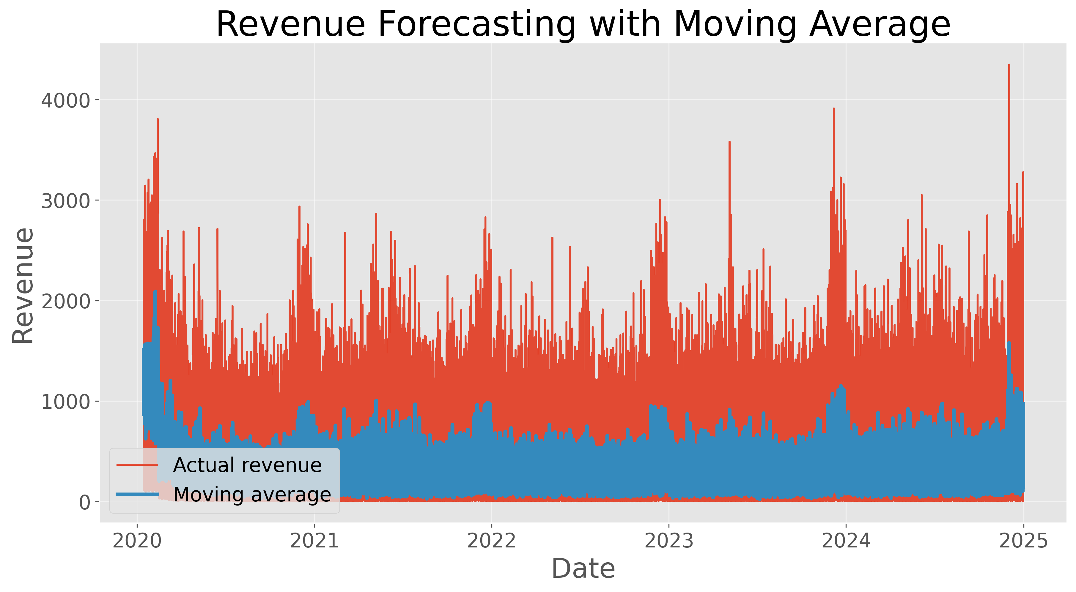
While noise cannot be predicted directly, analysts attempt to minimize its influence when building forecasting models. Techniques such as smoothing methods, moving averages, and statistical filtering help reveal the underlying structure of the data by reducing the impact of random fluctuations.

Why These Components Matter

Separating these four components allows analysts to better understand what is actually driving revenue changes.

In simplified form, a revenue time series can be represented as:

Observed Revenue= Trend + Seasonality + Cycles + Noise

Forecasting models attempt to estimate the predictable components—trend and seasonality—while minimizing the effect of noise. This decomposition helps analysts produce projections that reflect the true dynamics of the business rather than reacting to short-term irregularities.

Without this foundational understanding, forecasts can easily become misleading. A temporary spike might be mistaken for sustained growth, or a seasonal dip might be interpreted as declining demand.

For this reason, effective revenue forecasting always begins with a careful examination of the underlying time-series structure before selecting a modeling approach.

Building an Accurate Forecasting Model (Step-by-Step Approach)

Step 1: Collect and Structure Historical Sales Data

A forecasting model is only as reliable as its input data.

Best practices include:

• Use at least 24–36 months of historical sales data
• Maintain consistent time intervals (daily, weekly, or monthly)
• Segment revenue by meaningful dimensions when possible

Example dataset structure:

‍

Additional variables can also improve forecasts:

• marketing spend
• number of customers
• product category revenue
• pricing changes

Regression-based forecasting models can use these factors to predict revenue relationships.

Step 2: Explore and Visualize the Data

Before building a model, analysts should explore the historical data to identify patterns.

Typical exploratory steps include:

• plotting revenue trends over time
• identifying seasonal spikes
• detecting outliers or anomalies
• decomposing time-series components

Visualization tools such as Python (Matplotlib), Power BI, or Tableau make these patterns easier to interpret.

Example insight:

“Revenue consistently increases during Q4, indicating a seasonal pattern that must be incorporated into the forecast.”

Step 3: Choose an Appropriate Forecasting Model

There are several forecasting methods available, each designed to address different types of data patterns and analytical needs. The most appropriate method depends largely on the complexity of the underlying data as well as the length of the forecasting horizon. Simple approaches such as moving averages or basic trend projections may work well for stable datasets with minimal variability and short-term forecasting needs. However, more complex environments—where revenue is influenced by seasonal patterns, external business drivers, or long-term structural changes—often require more advanced techniques such as regression models or time-series methods.

Selecting the right forecasting approach therefore involves evaluating both the structure of the historical data and the time frame over which predictions are required. Below are the most common techniques:

1. Straight-Line Forecasting (Simple Growth Model)

The simplest revenue forecasting method assumes that revenue will continue to grow at a consistent rate over time. Under this approach, analysts examine historical growth patterns and apply the same rate of increase to future periods to estimate upcoming revenue. While this method is easy to implement and useful for quick projections, it works best when the business environment is relatively stable and past growth trends are expected to continue without significant disruption.

Example:

Forecast Revenue = Current Revenue × (1 + Growth Rate)


If revenue is $10M and the historical growth rate is 8%:

Next Year Forecast = $10M × 1.08 = $10.8M


This method is useful for early-stage forecasting or baseline projections.

2. Moving Averages and Exponential Smoothing

Moving averages smooth historical data by calculating the average revenue across multiple time periods, which helps reduce the influence of short-term fluctuations or random variation in the dataset. By dampening these temporary spikes and dips, moving averages reveal the underlying trend in revenue performance and provide a more stable foundation for generating forecasts.

Example:

3-month moving average
Forecast = (Month1 + Month2 + Month3) / 3


Exponential smoothing improves this approach by giving more weight to recent data.

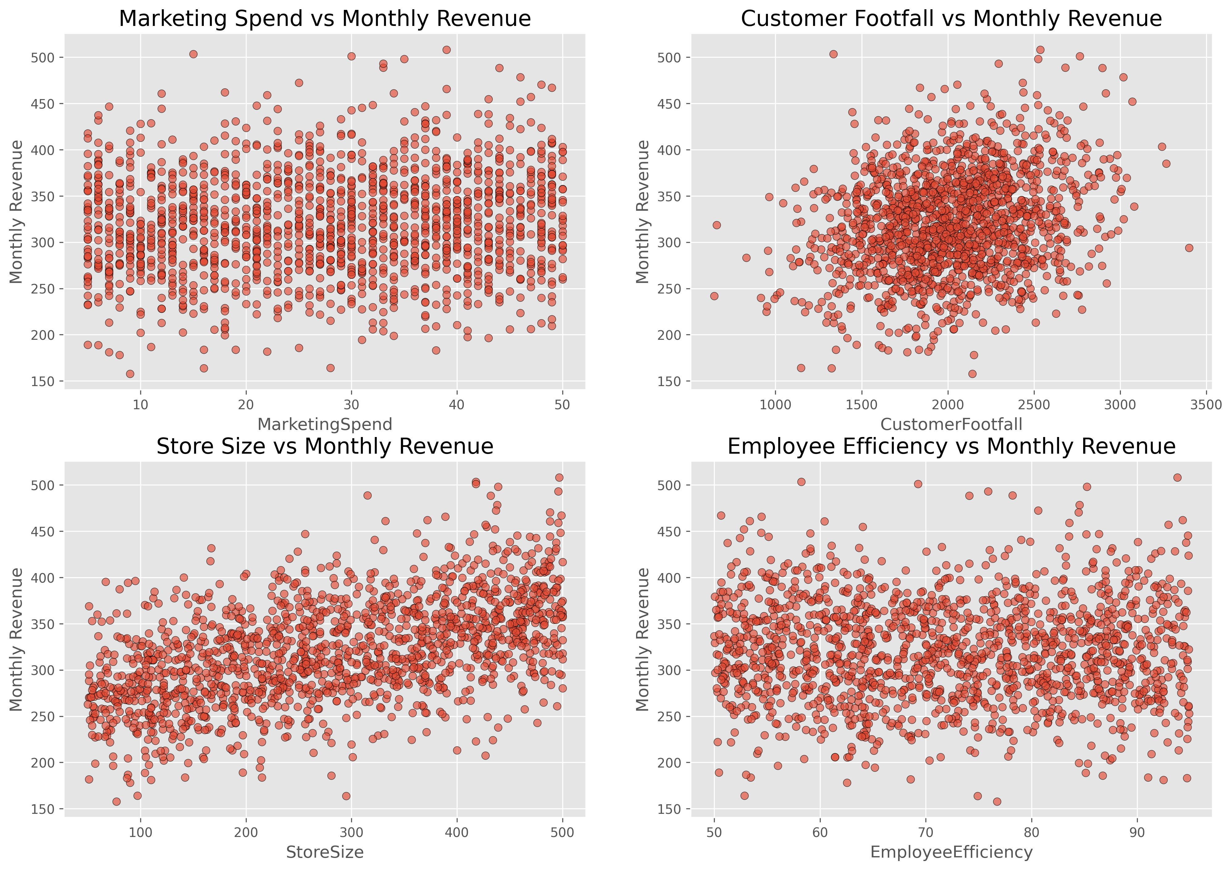
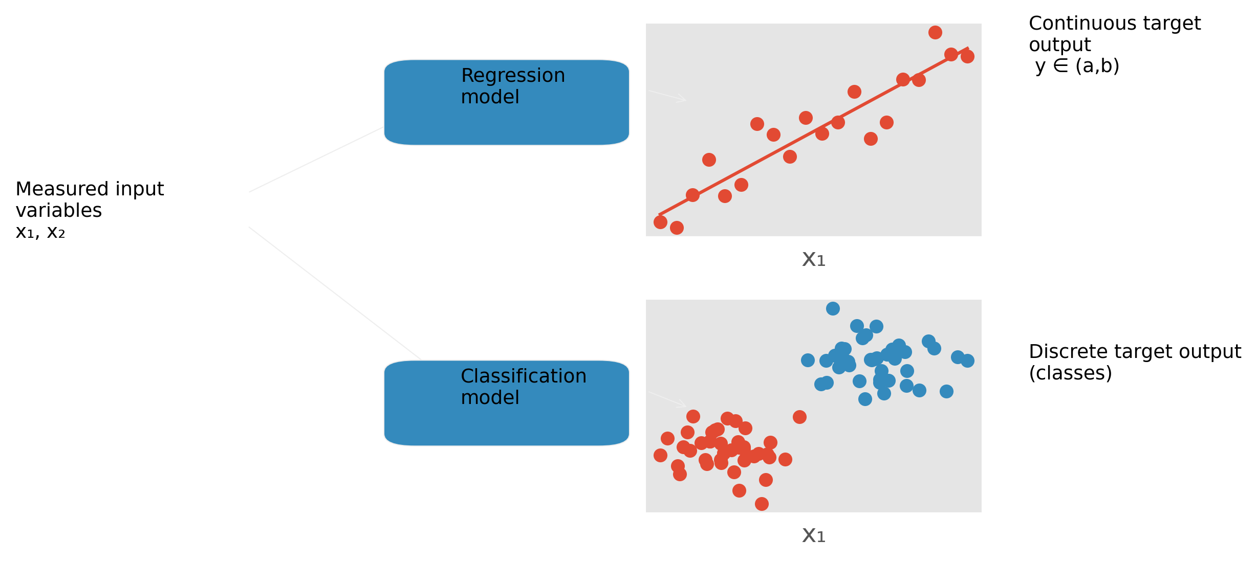
3. Regression-Based Forecasting

Regression models estimate the relationship between revenue and external variables that may influence sales performance. Instead of relying solely on historical revenue trends, regression analysis examines how factors such as marketing spend, pricing changes, customer traffic, or economic conditions affect revenue outcomes. By quantifying these relationships statistically, regression models allow analysts to understand which variables have the strongest impact on revenue and to generate forecasts based on expected changes in those drivers.

Example model:

Revenue = β0 + β1(Marketing Spend) + β2(Website Traffic) + ε


This approach is particularly valuable when revenue is strongly influenced by operational drivers like advertising spend or pricing changes.

4. Time-Series Models (ARIMA / SARIMA)

ARIMA (AutoRegressive Integrated Moving Average) is one of the most widely used statistical forecasting models.

It works by modeling relationships between past observations in the time series and projecting them forward.

Variants include:

• ARIMA — captures trends and autocorrelation
• SARIMA — incorporates seasonal patterns
• ETS (Exponential Smoothing) — ideal for trend + seasonality

These models are commonly used for monthly revenue forecasting and demand planning.

Step 4: Train and Validate the Model

A good forecasting model must be tested against historical data to measure its accuracy before it can be relied upon for decision-making. This process, often referred to as model validation, involves comparing the model’s predictions to actual historical outcomes in order to determine how well it captures the underlying patterns in the data. Analysts typically train the model using a portion of historical data and then evaluate its performance on a separate set of observations that were not used during training. By testing how closely the predicted values align with the real revenue figures, analysts can assess whether the model is producing meaningful forecasts or simply overfitting to past data.

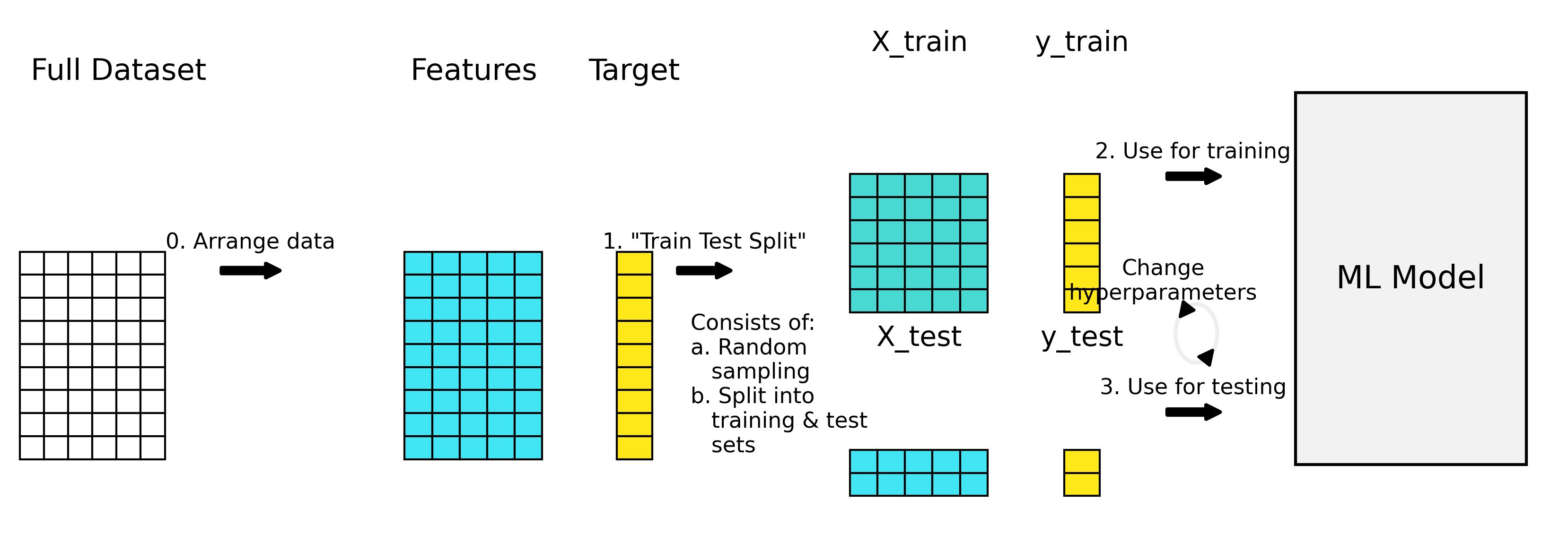
The standard workflow is:

1. Split data into training and testing sets
2. Train the model on historical data
3. Predict future values
4. Compare predicted vs actual results

This process allows analysts to evaluate forecasting performance before deploying the model in production.

Common evaluation metrics such as Mean Absolute Error (MAE), Root Mean Squared Error (RMSE), or Mean Absolute Percentage Error (MAPE) help quantify forecasting accuracy and allow different models to be compared objectively. Through this validation process, analysts can refine their forecasting approach, adjust model parameters, and ultimately select the model that provides the most reliable predictions for future revenue.

Step 5: Generate Forecast Scenarios

The best forecasting models provide multiple possible scenarios rather than a single number.

Typical forecast ranges include:

Scenario modeling helps leadership teams understand risk and plan for uncertainty.

Tools and Technologies for Revenue Forecasting

Several tools can be used to build revenue forecasting models, ranging from simple spreadsheet software to advanced analytics environments. The right tool typically depends on the complexity of the dataset, the forecasting horizon, and the level of statistical rigor required for the analysis. Simpler forecasting tasks can often be handled using spreadsheet applications such as Excel or Google Sheets, while more complex modeling workflows may require programming environments designed for statistical analysis.

For more advanced forecasting applications, analysts frequently rely on tools such as Python or R, which provide specialized libraries for time-series modeling, regression analysis, and machine learning forecasting. Business intelligence platforms like Power BI and Tableau are also commonly used to visualize historical trends and present forecast results through dashboards that support decision-making. In many organizations, effective forecasting workflows combine several of these tools to move from raw data to analytical insight and ultimately to strategic planning.

Excel / Google Sheets

Good for simple forecasts using built-in functions like:

FORECAST()
FORECAST.ETS()


These allow quick time-series projections using historical data.

Python (Recommended for Advanced Analytics)

Python offers powerful forecasting libraries:

Key libraries

• pandas (data manipulation)
• statsmodels (ARIMA, SARIMA)
• scikit-learn (regression models)
• Prophet (time-series forecasting)

Example workflow:

import pandas as pd
from prophet import Prophet

df = pd.read_csv("revenue.csv")

df = df.rename(columns={"date":"ds","revenue":"y"})

model = Prophet()
model.fit(df)

future = model.make_future_dataframe(periods=12, freq='M')
forecast = model.predict(future)


Python is widely used because it enables:

• automated model training
• statistical evaluation
• advanced machine learning forecasting

Power BI / Tableau

These tools allow analysts to:

• visualize revenue trends
• display forecast projections
• build executive dashboards

Power BI includes built-in forecasting for time-series charts, making it useful for operational reporting.

Best Practices for Accurate Forecasting

Even the most sophisticated forecasting models can produce unreliable results if they are built on weak foundations. Accurate revenue forecasting depends not only on statistical methods, but also on disciplined data practices and thoughtful model design. The following best practices help ensure that forecasts reflect meaningful business signals rather than artifacts of poor data or flawed assumptions.

1. Use Clean Historical Data

The quality of a forecasting model is fundamentally limited by the quality of the data used to train it. If historical revenue records are incomplete, inconsistent, or incorrectly structured, the model will learn patterns that do not reflect the true performance of the business.

Common data quality issues include:

• missing revenue values
• duplicate transactions
• inconsistent date formats
• revenue recorded in different currencies without normalization
• backdated corrections or accounting adjustments

For example, if several months of revenue data are missing or misreported, a model may interpret the gap as a sudden decline in demand rather than a data error. Similarly, a large one-time transaction may create an artificial spike that distorts the perceived trend.

Before building any forecasting model, analysts should perform basic data validation steps such as:

• verifying that revenue totals match financial reporting systems
• checking for missing time periods in the dataset
• removing or flagging obvious outliers
• ensuring consistent time intervals (daily, weekly, or monthly)

A clean and well-structured dataset allows the forecasting model to identify genuine patterns rather than reacting to data artifacts.

2. Incorporate Business Drivers

While historical revenue trends can provide valuable signals, revenue is rarely determined by time patterns alone. In many businesses, operational and strategic decisions significantly influence sales performance.

Examples of important business drivers include:

• marketing spend and advertising campaigns
• pricing adjustments or discounts
• product launches
• sales team expansion
• promotional events or seasonal sales initiatives

For instance, a sudden increase in marketing investment may lead to higher lead generation and sales conversions in subsequent months. If a forecasting model relies only on historical revenue without accounting for this change in marketing activity, it may underestimate future revenue growth.

Incorporating these drivers into forecasting models allows analysts to build causal relationships rather than relying purely on historical patterns. Regression models and machine learning approaches are particularly effective for modeling how these variables influence revenue.

By including relevant operational inputs, forecasts become more responsive to the real mechanisms that drive business performance.

3. Update Forecasts Regularly

Forecasts are not static predictions; they should evolve as new data becomes available. Markets change, customer behavior shifts, and internal strategies adapt. As a result, models trained on older data may gradually lose accuracy if they are not recalibrated.

A common practice is to update forecasts on a monthly or quarterly basis, incorporating the most recent revenue data into the model. This process allows the model to learn from new patterns and adjust projections accordingly.

Regular forecast updates provide several advantages:

• improved responsiveness to changing market conditions
• more accurate short-term projections
• early detection of performance deviations

For example, if revenue begins declining unexpectedly, updating the model with recent data allows analysts to quickly identify whether the change represents a temporary fluctuation or a more sustained trend.

Organizations often implement rolling forecasts, where each new month of data replaces the oldest period in the training dataset. This approach ensures that the forecasting model always reflects the most relevant historical information.

4. Compare Multiple Models

No single forecasting method performs best across all datasets or business environments. Different models capture different aspects of revenue behavior, and their effectiveness depends on the structure of the underlying data.

For example:

• moving averages may perform well for stable revenue streams with minimal volatility
• exponential smoothing methods are effective for capturing trends and seasonality
• regression models are useful when revenue is strongly influenced by external variables
• machine learning models can capture complex nonlinear relationships

Rather than relying on a single model, analysts often test several approaches and evaluate their performance using historical validation techniques. Metrics such as Mean Absolute Error (MAE), Root Mean Squared Error (RMSE), or Mean Absolute Percentage Error (MAPE) allow analysts to compare how accurately each model predicts known historical outcomes.

By comparing multiple models, analysts can identify the approach that best captures the structure of their revenue data. In many cases, combining forecasts from several models—known as ensemble forecasting—can produce even more stable results.

Final Thoughts

Revenue forecasting transforms historical sales data into forward-looking business intelligence. By combining time-series analysis, regression modeling, and modern analytics tools, organizations can produce forecasts that guide strategic decisions with far greater confidence.

The most effective forecasting models are not necessarily the most complex; instead, they are built on high-quality historical data that accurately reflects past business performance. They also incorporate relevant business drivers, such as pricing changes, marketing investment, or customer demand signals, so that forecasts reflect the real factors influencing revenue. Finally, strong forecasting models are continuously validated and improved, with analysts regularly testing predictions against new data and refining the model to maintain accuracy over time.

When implemented correctly, a revenue forecasting model becomes one of the most powerful analytical assets an organization can build.